Learning distribution-free anchored linear structural equation models in the presence of measurement error

This post is the summary of Chung, J., Ahn, Y., Shin, D., & Park, G. (2024). Learning distribution-free anchored linear structural equation models in the presence of measurement error. Journal of the Korean Statistical Society, 1-25.

Objective

This study aims to establish an identifiability in distribution-free anchored linear structural equation models(SEMs), where the observed variables are imperfect measures for the target variables. Based on the identifiability condition, a consistent learning algorithm of the complete partial directed acyclic graph(CPDAG) is developed.

Contributions

Establishes an identifiability condition of distribution-free anchored linear SEMs based on the geometry-faithfulness assumption.
Proposes a consistent learning algorithm to discover a latent structure in the presence of measurement error.
Provides various numerical experiments and analysis of real galaxy data.

Introduction

Identifiability of directed acyclic graphical models (DAG) is usually achieved by posing additional assumptions. For example,
- Causal minimality: True graph is a minimal structure that is Markov to its distribution.
- Faithfulness: Conditional independence implies d-separation.
  - Distributional constraints: Gaussian errors with equal variance (Peters and Bühlmann, 2014), non-Gaussian errors (Shimizu et al., 2006), etc.
The aforementioned identifiability results work under causal sufficiency regime, excluding the presence of latent variables.
However, in many real-world setting, observed variables are imperfect measures of corresponding true variables.

Motivating example

The above figure visualizes the relationship between the latent variables $X$ and the observed variables $Z$.
One can observe that $X_1$ and $X_3$ are d-separated(blocked) by $X_2$, while the statement becomes false if we replace $X$ to $Z$.

Linear structural equation model

A linear structural equation model(SEM) is a DAG model where the joint distribution is defined by the following linear equations: For all $j \in V$,
\[X_j = \sum_{k \in \text{Pa}(j)} \beta_{kj}X_k + \epsilon_j ,\]
where each $\epsilon_j$ is an independent, but possibly not identical error with mean $0$ and variance $\sigma_j^2$.
The above The linear SEM can be restated as a matrix form:
\[X = BX + \epsilon .\]
We denote $\mathcal{L}(G,B,F)$ as the linear SEM where $B$ is the edge weight matrix, $G$ is the underlying true DAG, and $\epsilon \sim F$.

Anchored linear structural equation model

An anchored DAG model considers a DAG model with latent variables.
In our framework, we consider an anchored linear SEM, special case of an anchored DAG model, as follows: For all $j \in V$,
\[Z_j = f_j(X_j) \quad \text{and} \quad X \sim \mathcal{L}\left(G,B,(0,\Sigma_\epsilon)\right) ,\]
where $\Sigma_\epsilon = \text{diag}(\sigma_1^2,…,\sigma_p^2)$, and $f_j : \mathbb{R} \to \mathbb{R}$ can be linear, non-linear, or even non-deterministic function.
- (Additive measurement error model) $f_j(X_j) = X_j + \psi_j$, where $\psi_j \sim (0,\eta_j^2)$.
- (Dropout model) $f_j(X_j) = X_j\psi_j$, where $\psi_j \sim \text{Bernoulli}(p)$.
- (Poisson transformation) $f_j(X_j) = \text{Poisson} ( \lvert X_j \rvert )$.

Identifiability

Geometry-faithfulness

Assumption 1(Geometry-faithfulness).

Consider a linear SEM $\mathcal{L}(G, B, (0, \Sigma_\epsilon))$ that generates $P(X)$, i.e., $X \sim \mathcal{L}(G, B, (0, \Sigma_\epsilon))$. Then, for any pair of nodes $j, k \in V$, and for any subset $S \subset V \setminus \{j, k\}$:
\[\text{$j$ and $k$ are d-separated by $S$ in $G$} \iff \rho_{j,k,S} \propto [(\Sigma_{L,L})^{-1}]_{j,k} = 0,\]
where

$\Sigma = (I_p - B)^{-1}\Sigma_{\epsilon}(I_p - B)^{-\top}$,

$L = S \cup \{j, k\}$, and

$\rho_{j,k,S}$ is the partial correlation coefficient of $X_j$ and $X_k$ given $X_S$.

Geometry-faithfulness ensures that partial correlations directly reflect d-separations and connections within the graph.
Under the geometry-faithfulness assumption, $j$ and $k$ are d-separated by $S$ if and only if the residuals obtained by projecting $X_j$ and $X_k$ onto $X_S$ are orthogonal.
This assumption is violated only at the same parameter set of measure zero as the faithfulness assumption is.

Identifiability

Theorem 1(Identifiability for distribution-free anchored linear SEMs).

Consider a distribution-free anchored linear SEM with $\mathcal{L}\left(G, B, (0, \Sigma_{\epsilon})\right)$.
Then, the model is identifiable up to the MEC if the following conditions are satisfied:

(A1): The latent distribution $P(X)$ is geometry-faithful to $G$.

(A2): The observed random variables satisfy the following condition:
For all $j \in V$, $Z_j \perp \{Z_1, \dots, Z_p, X_1, \dots, X_p\} \setminus \{ Z_j, X_j \} \mid X_j.$

(A3): For all $j, k \in V$:

There exists a finite-dimensional vector $\delta_j$ of monomials in $Z_j$ and a finite-dimensional vector $\delta_{jk}$ of monomials in $Z_j$ and $Z_k$,

Their means can be mapped to the moments of the latent variables by continuously differentiable functions $g_j$, $g_{jj}$, and $g_{jk}$, such that: $\mathbb{E}[X_j] = g_j(\mathbb{E}[\delta_j]),$ $\mathbb{E}[X_j^2] = g_{jj}(\mathbb{E}[\delta_{jj}]),$ $\mathbb{E}[X_j X_k] = g_{jk}(\mathbb{E}[\delta_{jk}]),$

The covariance satisfies: $\mathrm{Cov}(\delta_j, \delta_{jk}) < \infty.$

Theorem 1 is motivated from Saeed et al. (2020), while they require the errors to be Gaussian as it uses the faithfulness assumption.
However, our theorem bypasses the need of distributional constraints by introducing the geometry-faithfulness assumption.

Algorithm

Algorithm 1(CPDAG learning algorithm for distribution-free anchored linear SEMs).

Input:

$n$ i.i.d. observations from an anchored linear SEM, $Z^{1:n}$

Transformation $\mathcal{T}$ and function $g$ such that $\mathrm{Cov}(X) = \mathcal{T}\left(\mathbb{E}[g(Z)]\right)$

Significance level $\alpha$

Output:

Complete Partial DAG (CPDAG), $\widehat{G}_{cp}$

Steps:

Estimate the mean of $g(Z)$ from $Z^{1:n}$.

Estimate the covariance matrix $\hat{\Sigma}$ for latent variables using $\mathcal{T}$ and $g$.

Estimate the partial correlations of $X$ using $\hat{\Sigma}$.

Estimate a CPDAG using a constraint-based algorithm (e.g., the PC algorithm) by conducting a consistent partial correlation test with $\alpha$.

Return:

Estimated CPDAG, $\widehat{G}_{cp}$

Algorithm 1 is a statistically consistent algorithm for learning the CPDAG of a distribution-free anchored linear SEM, given that consistent estimators for the mean of $g(Z)$ and conditional independence tests are used.
This methodology also aligns with the algorithm proposed in Saeed et al. (2020).
However, the consistency of this approach under the distribution-free settings has not been explored previously.

Consistency

Theorem 2(Consistency)

Consider an anchored linear SEM with the true CPDAG $G_{cp}$. Suppose that the strong geometry-faithfulness assumption and Assumptions (A2)-(A3) are satisfied. Additionally, suppose that the sequence of signifcance level $\{\alpha_n : n \in \mathbb{N}\}$ satisfies $2\big(1-\Phi\big(0.5 \rho_{\min}\sqrt{n-p-1}\big)\big) < \alpha_n < 1$ for all $n \in \mathbb{N}$ where $\Phi(\cdot)$ denotes the CDF of $N(0,1)$. Then, Algorithm 1 is consistent, i.e.,
\[\widehat{G}_{cp} \to G_{cp} \quad \text{as} \quad n \to \infty ,\]
where $\widehat{G}_{cp}$ is the estimated CPDAG by Algorithm 1.

Based on Fisher’s z-test, Theorem 2 demonstrates that the proposed algorithm consistently learns a distribution-free anchored linear SEM under the sample version of the identifiability condition and with an appropriate choice of significance level.

Numerical experiments

Experiment settings

The simulation study was conducted by generating $100$ instacnes of random (i) dropout models, and (ii) additive measurement error models.
- For dropout models, the non-zero probability was uniformly set at $\gamma = 0.9$.
- For additive measurement error models, the variance of the measurement error was set at $\eta^2 = 0.25$.
In terms of error distributions, four sets of noise distributions were considered:
- Non-identical but symmetric distributions, where $\epsilon_j$ follows different distributions based on $j \mod 4$:
  - $\epsilon \sim N(0,1)$ for $j \equiv 1$,
  - $\epsilon \sim \text{Uniform}(-2,2)$ for $j \equiv 2$,
  - $\epsilon \sim t(15)$ for $j \equiv 3$,
  - $\epsilon \sim \text{Discrete Uniform}\{-1,1\}$ for $j \equiv 0$.
- All i.i.d. centered Gamma distributions with shape and scale parameters set to $1$,
- All i.i.d. centered Weibull distributions with shape and scale parameters set to $1$,
- All i.i.d. Gaussian distributions, $N(0,1)$.

Dropout models

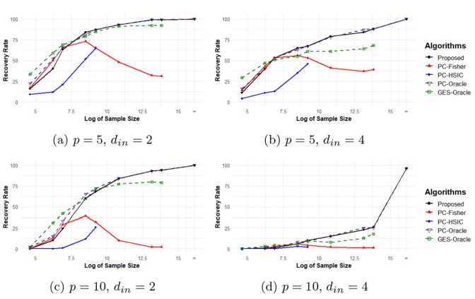
Figure 2: Comparison of the proposed algorithm to the PC-Fisher, PC-HSIC, PC-Oracle, and GES-Oracle algorithms with the first set of error distribution

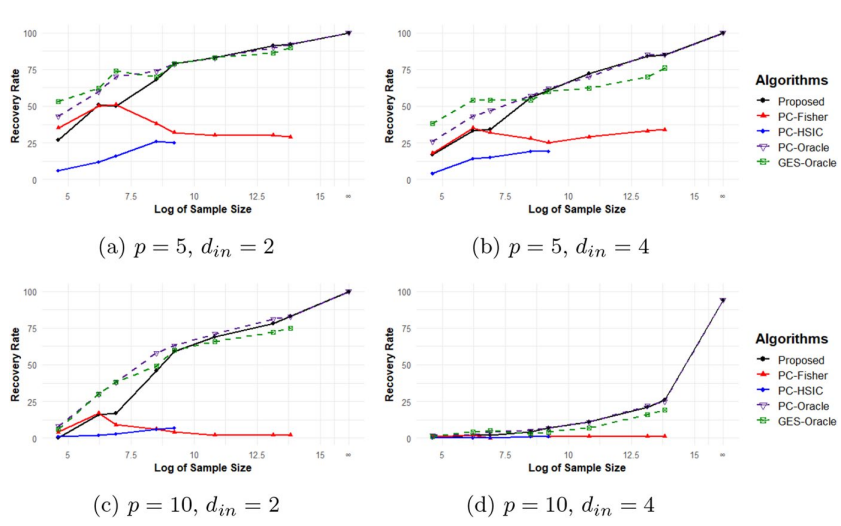
$d_{in}$ denotes the maximum indegree.
The result corroborates the consistency of the proposed algorithm.

Additive measurement error models

Figure 3: Comparison of the proposed algorithm to the PC-Fisher, PC-HSIC, PC-Oracle, and GES-Oracle algorithms with the first set of error distribution

The results in Figures 4 and 5 align closely with those for the dropout models shown in above.

Real data

Figure 4: Comparison between the true CPDAG and the estimated CPDAG by the proposed algorithm.

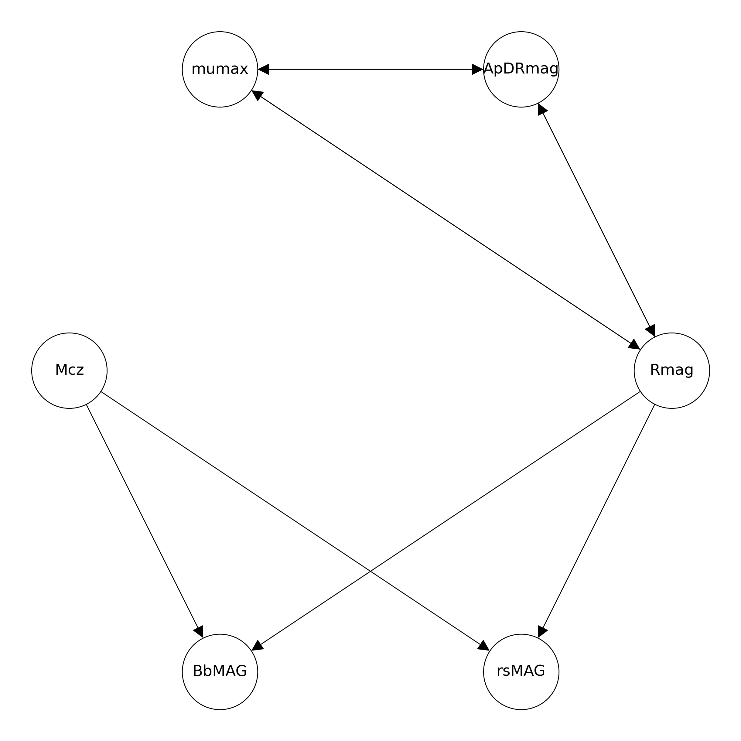
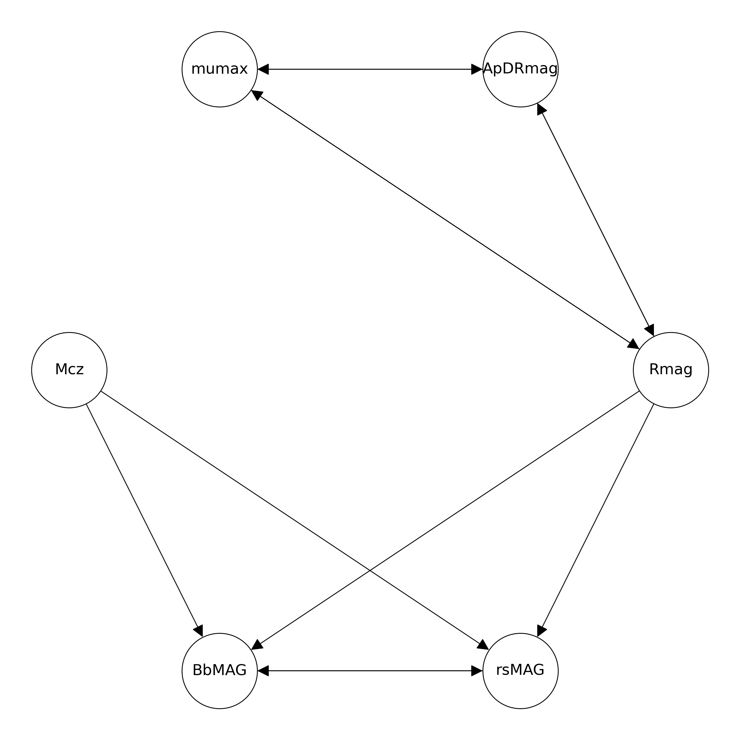
The data ($p = 6, n = 3462$) comprises galaxy brightness measurements, which also includes measurement errors for each variable.
- Rmag ($0.0069$), mumax ($0$), ApDRmag ($0$), Mcz ($0.0038$), BbMAG ($1.5233$) and rsMAG ($1.6508$).
The proposed algorithm successfully detects all true edges, while falsely detects an undirected edge (BbMAG, rsMAG).

References

Chung, J., Ahn, Y., Shin, D., & Park, G. (2024). Learning distribution-free anchored linear structural equation models in the presence of measurement error. Journal of the Korean Statistical Society, 1-25.
Halpern, Y., Horng, S., & Sontag, D. (2015). Anchored discrete factor analysis. arXiv preprint arXiv:1511.03299.
Liu, Y., Constantinou, A. C., & Guo, Z. (2022). Improving Bayesian network structure learning in the presence of measurement error. Journal of Machine Learning Research, 23(324), 1-28.
Peters, J., & Bühlmann, P. (2014). Identifiability of Gaussian structural equation models with equal error variances. Biometrika, 101(1), 219-228.
Saeed, B., Belyaeva, A., Wang, Y., & Uhler, C. (2020). Anchored causal inference in the presence of measurement error. In Conference on uncertainty in artificial intelligence (pp. 619-628). PMLR.
Shimizu, S., Hoyer, P. O., Hyvärinen, A., Kerminen, A., & Jordan, M. (2006). A linear non-Gaussian acyclic model for causal discovery. Journal of Machine Learning Research, 7(10).
Zhang, K., Gong, M., Ramsey, J., Batmanghelich, K., Spirtes, P., & Glymour, C. (2017). Causal discovery in the presence of measurement error: Identifiability conditions. arXiv preprint arXiv:1706.03768.
Zhang, K., Gong, M., Ramsey, J. D., Batmanghelich, K., Spirtes, P., & Glymour, C. (2018). Causal Discovery with Linear Non-Gaussian Models under Measurement Error: Structural Identifiability Results. In UAI (pp. 1063-1072).

PREVIOUSHorse race rank prediction using learning-to-rank approaches