This post is the summary of Shin, J., Chung, J., Hwang, S., & Park, G. (2025). Discovering Causal Structures in Corrupted Data: Frugality in Anchored Gaussian DAG Models. Computational Statistics & Data Analysis, 108267.
Objective
This study focuses on establishing a weaker form of identifiability for anchored Gaussian DAG models, where knowledge of the measurement error variance is unavailable. Based on the condition, sound learning algorithms of the complete partial directed acyclic graph(CPDAG) are devised.
Contributions
- Introduces the anchored-frugality assumption, leveraging the fact that contaminated data tend to produce a denser graph than the true graph.
- Provides theoretical justifications for the anchored-frugality assumption from both graph-theoretical and probabilistic perspectives.
- Develops two theoretically sound algorithms for anchored Gaussian DAG models, building upon and extending the sparsest permutation(SP) algorithm (Raskutti and Uhler (2018)) and the PC algorithm.
- Conducts comprehensive numerical experiments and application to breast cancer data and protein signaling data, supporting the main theoretical findings of the study.
Introduction
- Identifiability of directed acyclic graphical models is usually achieved by posing additional assumptions, most of which require variables to be directly observed.
- However, in many real-world settings, observed variables are imperfect measures of corresponding true variables.
- A number of studies have tackled this issue under anchored DAG models. For example,
- Zhang et al. (2017) propose a consistent algorithm when the number of leaf nodes is sufficiently small and the non-deterministic faithfulness holds, which is stronger than the standard faithfulness.
- Saeed et al. (2020) establish a PC-based algorithm that achieves consistency when the latent variables are Gaussian and the contamination process is known.
- Chung et al. (2024) develop a consistent distribution-free algorithm when the contamination process is given.
- This highlights the need for an algorithm that (i) works under more relaxed conditions and (ii) does not require the contamination process to be known.
Preliminaries
Directed acyclic graph
- A DAG $G = (V,E)$ consists of a set of nodes $V = \{1,…,p\}$ and a set of directed edges $E \subset V \times V$ with no directed cycles.
- A skeleton of a DAG $G$ is attained by replacing all directed edges to undirected edges, and we denote $\vert G \vert$ for the number of edges in its skeleton.
- A set of parents of node $k$, denoted by $\text{Pa}(k)$, consists of all nodes $j$ such that $(j,k) \in E$.
- If there is a directed path $j \rightarrow \cdots \rightarrow k$, then $k$ is a descendant of $j$, and $j$ is called an ancestor of $k$.
- A node $k$ is a collider if there exists a triple $(j,k,\ell)$ such that $j \rightarrow k \leftarrow \ell$, and we say such triple generates a v-structure.
D-separation and d-connection
- Two nodes $j$ and $k$ in DAG $G$ are d-connected by a node set $S \subset V$ if there exists a path $\mathcal{P}$ between $j$ and $k$ such that for every node $\ell$ on the path $\mathcal{P}$,
- if $\ell$ is a collider, either $\ell$ or its descendant is in $S$,
- otherwise $\ell$ is not in $S$.
- If $j$ and $k$ are not d-connected by $S$, we say $j$ and $k$ are d-separated by $S$.
Markov equivalence class
- Two DAGs $G_1$ and $G_2$ are Markov equivalent if they have the same skeleton and the same set of v-structures. We simply denote $G_1 \overset{\text{M.E.}}{\sim} G_2$ if $G_1$ and $G_2$ are Markov equivalent.
- A Markov equivalence class(MEC) of $G$, denoted by $M(G)$, is the set of all DAGs that are Markov equivalent to $G$.
Anchored DAG
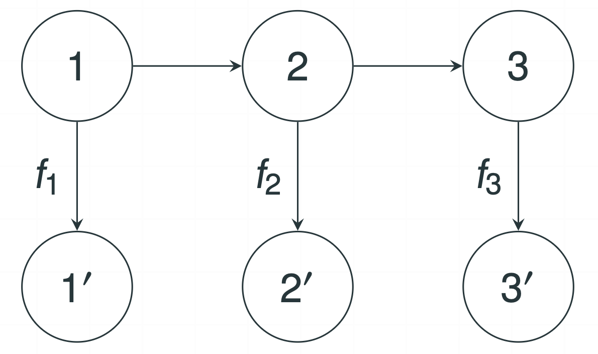
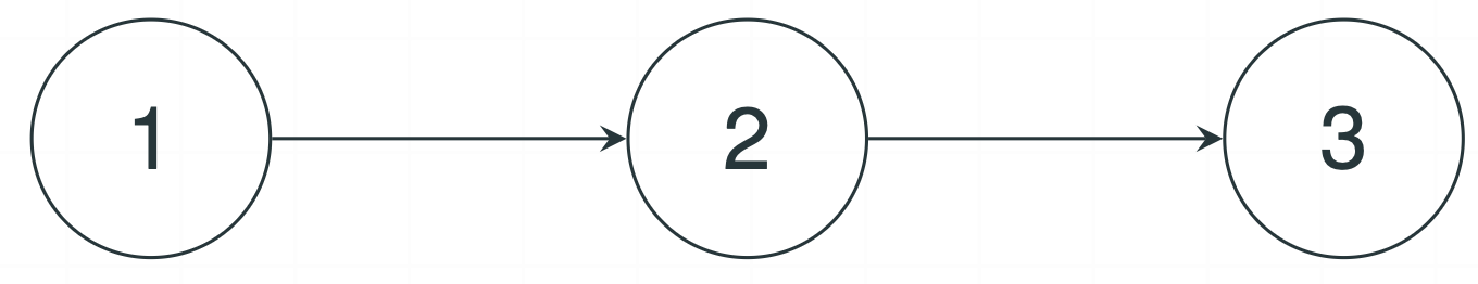
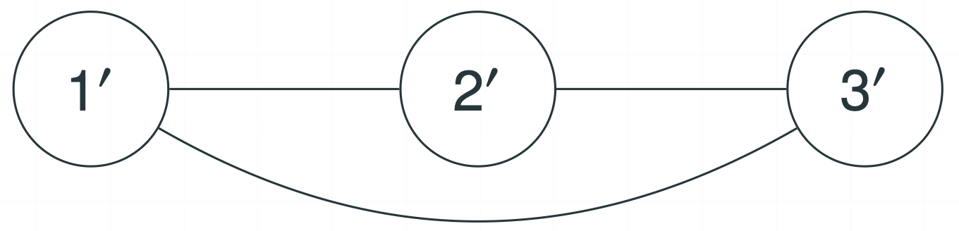
Figure 1: Illustration of three graphical representations in an anchored DAG model
- An anchored DAG for $G = (V,E)$ is denoted as $G_{an} = (V_{an},E_{an})$.
- $V_{an} = V \cup V^\prime$, where $V^\prime = \{1^\prime,…,p^\prime\}$ represents the vertex set of anchored nodes. Here, $j^\prime$ is the anchored node corresponding to $j$, i.e., $\text{Pa}(j^\prime) = \{j\}$ for each $j \in V$.
- $E_{an} = E \cup \{(j,j^\prime): j \in V\}$.
- An anchored moral graph of $G$ is an undirected graph defined by the vertex set $V^\prime$ and $E^\prime$, where
- $E^\prime = \{(j^\prime,k^\prime): \text{$j^\prime$ and $k^\prime$ cannot be d-separated by any subset $S^\prime \subset V^\prime \setminus \{j^\prime,k^\prime\}$}\}$.
- Intuitively, the anchored moral graph serves as a corrupted representation for $G$, obtained with obfuscated data.
Anchored Gaussian linear structural equation model
-
A Gaussian linear structural equation model(SEM) is a Gaussian DAG model where the joint distribution is defined by the following linear equations: For all $j \in V$,
\[X_j = \sum_{k \in \text{Pa}(j)} \beta_{kj}X_k + \epsilon_j ,\]where $\epsilon_j \overset{\text{indep.}}{\sim} N(0,\sigma_j^2)$.
-
The above linear SEM can be restated as a matrix form:
\[X = BX + \epsilon .\] -
In our framework, we focus on an Gaussian additive measurement error model, which is the special case of an anchored Gaussian linear SEM. Precisely, for all $j \in V$,
\[Z = X + E ,\]where $E \sim N(0,\text{diag}(\eta_1^2,…,\eta_p^2))$. Then, $\Sigma_Z = \Sigma_X + \text{diag}(\eta_1^2,…,\eta_p^2)$.
-
Our goal is to recover the true DAG of $X$ using only $Z$.
Identifiability
Anchored-frugality
Assumption 1(Anchored-frugality).
Consider an Gaussian additive measurement error model, in which the true distribution of the latent variable $X$ is equal to $P_\eta \sim N(0, \Sigma_Z - \text{diag}(\eta_1^2,…,\eta_p^2))$. A pair $(G,P(X)) = (G,P_\eta)$ is said to satisfy the anchored-frugality assumption if for each valid $\lambda \in [0,\lambda_\min(\Sigma_Z))^p$, it holds either $\vert G_\lambda \vert > \vert G \vert$ or $G_\lambda \overset{\text{M.E.}}{\sim} G$, where $G_\lambda$ is any DAG that satisfies the Markov condition for $P_\lambda$.
- The anchored-frugality assumption posits that any DAG induced by distributions with unremoved measurement error variance is always denser than the true graph.
- This assumption leads to an algorithm that selects the sparsest graph among the candidate distributions as an estimator for the true graph.
Theorem 1 (Identifiability).
Consider an Gaussian additive measurement error model, and suppose that the anchored-frugality assumption is satisfied. Then, the model is identifiabile up to its MEC.
- Theorem 1 requires neither the knowledge of the measurement error variance nor the conventional faithfulness.
Rationales behind anchored-frugality
Graph theory
Lemma 1 (Frugality property).
Consider an anchored DAG $G_{an} = (V_{an},E_{an})$.
- If a pair of latent nodes is d-connected, the corresponding pair of anchored nodes is also d-connected by any set of anchored nodes.
- If a pair of latent nodes is d-separated due to no path between them, the corresponding pair of anchored nodes is also d-separated by any set of anchored nodes.
- If a pair of latent nodes is d-separated due to the presence of a collider in the path between them, the corresponding pair can be d-connected by some anchored nodes.
- Lemma 1 states that $j^\prime$ and $k^\prime$ are adjacent in the anchored moral graph if $j$ and $k$ are d-connected.
- This implies that the true graph is generally sparser that its corresponding anchored moral graph.
Corollary 1 (Relationship with standard faithfulness).
Consider a DAG model $(G,P(X))$ and its corresponding anchored DAG model $(G_{an},P(X,X^\prime))$, where $X$ is a latent random vector and $X^\prime = (F_1(X_1),…,F_p(X_p))^T$ is a transformed random vector. Suppose that $P(X,X^\prime)$ is faithful to $G_{an}$. Then, for any $G^\prime$ that satisfies Markov condition for $P(X^\prime)$, it holds that
- the skeleton $G^\prime$ is the supergraph of that of $G$, and
- $\vert G \vert = \vert G^\prime \vert$ if and only if $G \overset{\text{M.E.}}{\sim} G^\prime$.
- Corollary 1 demonstrates that the anchored-frugality assumption is implied by the standard faithfulness assumption.
Probability theory
Lemma 2 (Frugality property).
Consider a $p$-variate Gaussian distribution $P_\lambda \sim N(0, \Sigma - \text{diag}(\lambda_1^2,…,\lambda_p^2))$ where $\lambda \in \mathbb{R}^p$ and $\Sigma \in \mathbb{R}^{p \times p}$ is positive definite. Let $X_\lambda^\prime$ be a random vector such that $X_\lambda^\prime \sim P_\lambda$. For ease of notation, we additionally define $\Lambda_\Sigma = [0,\lambda_\min(\Sigma))^p$. Then, for any $j,k \in V$ and any $S \subset V \setminus \{j,k\}$, only one of the following three holds:
- $X_{\lambda,j}^\prime \perp\!\!\!\perp X_{\lambda,k}^\prime \mid X_{\lambda,S}^\prime$ for all $\lambda \in \Lambda_\Sigma$.
- $X_{\lambda,j}^\prime \not\!\perp\!\!\!\perp X_{\lambda,k}^\prime \mid X_{\lambda,S}^\prime$ for all $\lambda \in \Lambda_\Sigma$.
- There exists a non-empty Lebesgue measure zero set $\Lambda_\Sigma^{(j,k \mid S)} \subset \Lambda_\Sigma$ such that $X_{\lambda,j}^\prime \perp\!\!\!\perp X_{\lambda,k}^\prime \mid X_{\lambda,S}^\prime$ only for $\lambda \in \Lambda_\Sigma^{(j,k \mid S)}$ while $X_{\lambda,j}^\prime \not\!\perp\!\!\!\perp X_{\lambda,k}^\prime \mid X_{\lambda,S}^\prime$ for $\lambda \in \Lambda_\Sigma \setminus \Lambda_\Sigma^{(j,k \mid S)}$.
- Lemma 2 confirms that the anchored-frugality assumption is violated on a set of measure zero.
Algorithm
Algorithm
Algorithm 1 (Frugal-PC algorithm for Gaussian additive measurement error models with i.i.d. measurement errors).
Input:
- $n$ i.i.d. observations from a additive Gaussian measurement error model, $Z^{1:n}$
- The number of grids, $\tau$
Output:
- Complete partial DAG (CPDAG), $\hat{G^{cp}}$
Steps:
- Estimate the covariance matrix $\Sigma_Z = E(ZZ^T)$
- Set $\mathcal{E} \subset [0,\lambda_\min(\Sigma_Z))$ such that $\vert \mathcal{E} \vert = \tau$
- for $\eta^{\prime} \in \mathcal{E}$ do
- Calculate the partial correlations of $X$ from $\Sigma_{\eta^{\prime}} = \Sigma_Z * \eta^{\prime 2} I_p$
- Recover the CI relations using the partial correlations
- Estimate a CPDAG, $\hat{G^{cp}_{\eta^{\prime}}}$ using the PC algorithm based on the CI relations
- Determine the sparsest \(\hat{G^{cp}_{\hat{\eta}}}\) as $\hat{G^{cp}}$ where $\hat{\eta} = \arg\min_{\eta^{\prime}} \vert \hat{G^{cp}_{\eta^{\prime}}} \vert$
Return:
- Estimated CPDAG, \(\hat{G^{cp}}\)
Theoretical guarantees
Theorem 2 (Soundness).
Consider a Gaussian additive measurement error model with i.i.d. measurement errors. Under appropriate choice of $\mathcal{E}$ and some assumptions, Algorithm 1 returns the true CPDAG of the latent variables.
Corollary 1 (Consistency).
Under appropriate conditions and with the proper choice of estimators and tests, Algorithm 1 asymptotically finds the true CPDAG as sample size grows to infinity.
Numerical experiments
Experiment settings
- The simulation study was conducted by generating 100 instances of Gaussian additive measurement error models.
- The variance of the measurement error was set at $\eta^2 = 0.25$.
- True graphs were generated at random while respecting the pre-determined maximum indegree $d_{in} \in \{1,2,3\}$.
- Throughout the experiments, the number of grids was fixed at $\tau = 100$, and each element in $\mathcal{E}$ was evenly spaced.
Results
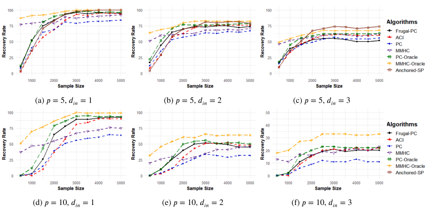
Figure 2: Comparison of the proposed Anchored-SP and Frugal-PC algorithms to the ACI, PC, MMHC, PC-Oracle, and MMHC-Oracle algorithms in terms of average graph recovery rate when recovering Gaussian additive measurement error models
- The Frugal-PC algorithm outperforms other algorithms in sparse settings, for which the anchored-frugality assumption is particularly well-suited.
- In dense settings, the Frugal-PC algorithm is still accurate as the ACI algorithm, benefiting from knowing the true value of $\eta^2$.
Real data
Data description
- The breast cancer dataset ($p=10$, $n=569$) collected by Street et al. (1993) consists of digitized images of fine needle aspirates of breast masses, described by 10 different types of features.
- After removing some redundant variables, the analysis was conducted with 8 variables, all of which were normalized to obviate scale-variant problem.
Original data
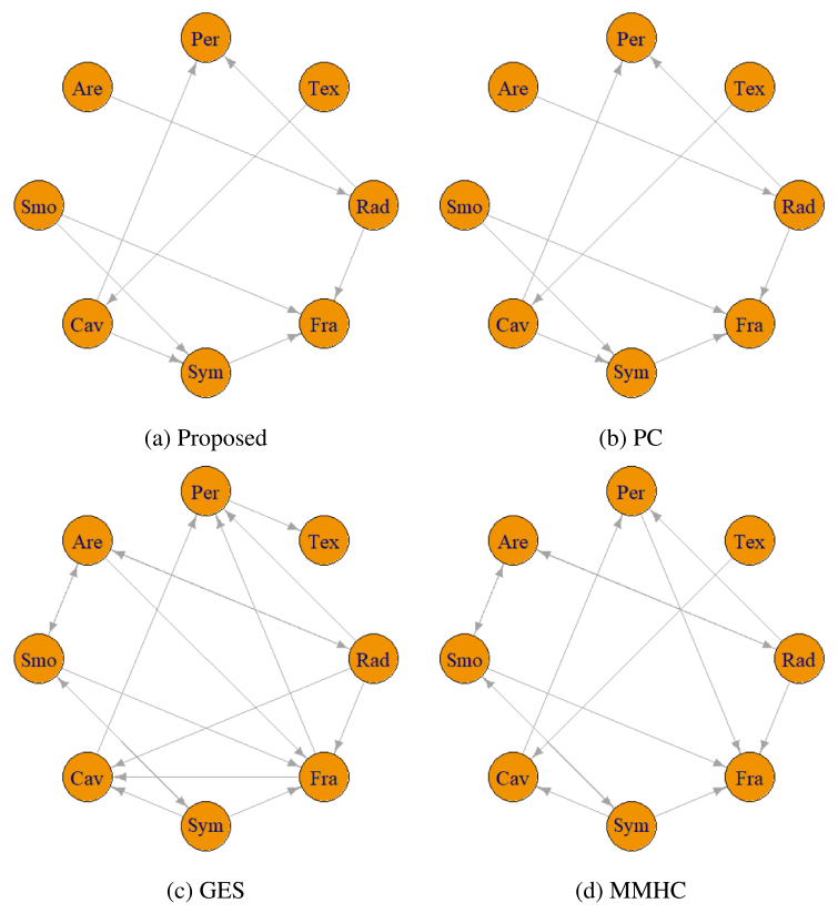
Figure 3: Estimated CPDAGs by the proposed Frugal-PC algorithm and the comparison PC, GES, MMHC algorithms with the original breast cancer data
- The ACI algorithm was omitted because the transformation is unknown.
- The Frugal-PC and PC algorithms yielded identical graphs, suggesting the measurement error in the data is negligible.
Perturbed data
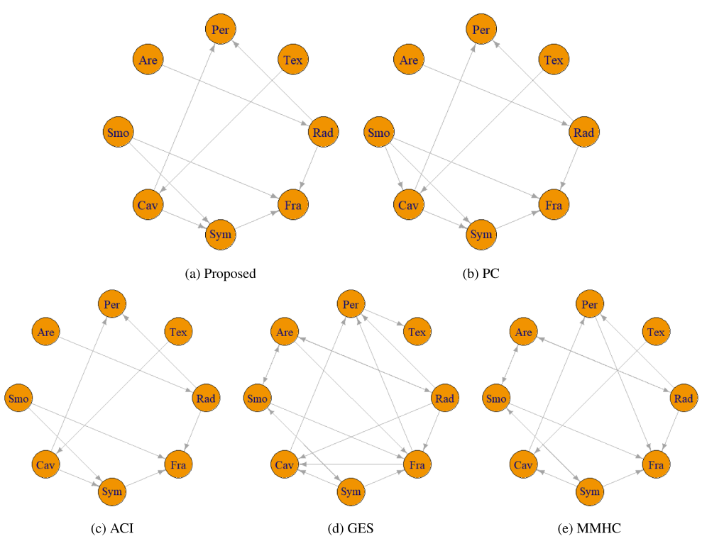
Figure 4: Estimated CPDAGs by the proposed Frugal-PC algorithm and the comparison ACI, PC, GES, MMHC algorithms with the perturbed breast cancer data
- To confirm the robustness of our algorithm against measurement error, we artificially perturbed the data by adding i.i.d. Gaussian random noise with $\eta^2 \approx 5 \times (0.1)^4$.
- It is remarkable that the proposed algorithm produced the same graph even in the presence of measurement error, whereas the PC algorithm detected a spurious edge (Smo, Cav).
- Moreover, the proposed algorithm successfully estimated $\eta$, yielding $\hat{\eta}^2 \approx 4 \times (0.1)^4$, guiding to an intriguing futre work on the estimation of measurement error variance.
References
- Chung, J., Ahn, Y., Shin, D., & Park, G. (2024). Learning distribution-free anchored linear structural equation models in the presence of measurement error. Journal of the Korean Statistical Society, 1-25.
- Raskutti, G., & Uhler, C. (2018). Learning directed acyclic graph models based on sparsest permutations. Stat, 7(1), e183.
- Saeed, B., Belyaeva, A., Wang, Y., & Uhler, C. (2020). Anchored causal inference in the presence of measurement error. In Conference on uncertainty in artificial intelligence (pp. 619-628). PMLR.
- Shin, J., Chung, J., Hwang, S., & Park, G. (2025). Discovering Causal Structures in Corrupted Data: Frugality in Anchored Gaussian DAG Models. Computational Statistics & Data Analysis, 108267.
- Street, W. N., Wolberg, W. H., & Mangasarian, O. L. (1993, July). Nuclear feature extraction for breast tumor diagnosis. In Biomedical image processing and biomedical visualization (Vol. 1905, pp. 861-870). SPIE.
- Zhang, K., Gong, M., Ramsey, J., Batmanghelich, K., Spirtes, P., & Glymour, C. (2017). Causal discovery in the presence of measurement error: Identifiability conditions. arXiv preprint arXiv:1706.03768.